Infection prevalence surveys estimate how many people are infected by testing a random sample of the population. I developed statistical methods for analysing these surveys [1] and worked on REACT-1 [2, 3, 4], which tested over 2.5 million swabs in England during COVID-19.
Statistical research
Daily survey results are noisy, so estimating trends from them requires a statistical model. However, we don’t want our results to be biased by implicit assumptions, and also want our uncertainty estimates to be well-calibrated. A range of such models were built during the pandemic. I stress-tested and improved two of them [5, 6], and compared the outputs with a model free of some of their assumptions [1].
The three models
Smoothing splines
Bayesian P-splines [5] represent the trend as a weighted sum of cubic B-spline basis functions centred on evenly spaced knots. Knot spacing limits how quickly the trend can change.
Fitted with Hamiltonian Monte Carlo in Stan.
Gaussian process
A Gaussian process [6] treats the trend’s values on any set of days as jointly Gaussian, correlated according to a squared-exponential kernel. The lengthscale determines how slowly correlation declines as the time between days increases.
Fitted with Hamiltonian Monte Carlo in Stan using a Hilbert space approximation to the Gaussian process [7].
Hidden-state with SMC
A hidden-state model [1] treats the trend as an unobserved random process. The step size is the standard deviation of the daily change in the trend’s slope.
Fitted with a particle filter inside particle marginal Metropolis–Hastings [8, 9].
Findings
Standard noise models are overconfident
The standard (binomial) model assumes that all day-to-day variation comes from sampling. Survey data vary more than that, so the model treats the extra noise as real changes in the trend. On REACT-1 data, its growth-rate estimates swung far more than those from a beta-binomial model [1]. This results in overconfidence in periods of data collection, and underconfidence in projections.
Smoothing parameters have real-world interpretations and should be estimated
Smoothing parameters are often hand-picked by the user and ignored, but they have real-world meanings and can (and should) be estimated from the data. In the hidden-state model, the smoothing parameter is the standard deviation of the daily change in the trend’s slope (the parameter slider above) [1]. Estimating this tells us how quickly the growth rate of COVID-19 was changing.
Use of statistical theory reduced runtimes substantially
The original splines model did not converge on the full REACT-1 dataset after 31 hours of computation. A better-fitting noise model, combined with architectural changes, reduced this to 39 minutes [1].
With statistical theory, we can fit the same underlying model using a particle filter: with daily knots, the splines model is equivalent to a random walk on the growth rate. This reduced the runtime to 4 minutes [1].
Real-time estimates should be in real-time
The splines-based method had to back-out the reproduction number (R) from its model. The additional assumptions involved resulted in estimates running ~1 week behind.
Our new hidden-state model can directly link new infections to prevalence, so can produce estimates in real time [1].
Data fusion enhances estimates
Only some positive swabs were genetically sequenced to identify the variant, because sequencing is slow and expensive. Analysing the sequenced swabs on their own throws away most of the data.
Our hidden-state model combines the sequencing results with the test results from every swab, so it can estimate how fast each variant was growing, with greater precision than alternative methods [1].
Applied analysis
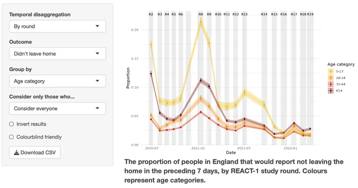
REACT-1 collected swab results and questionnaires from over 2 million people in England. Alongside the methods work, I analysed infection trends during the Omicron waves [2], led the analysis of how people’s behaviour changed over the pandemic [4], and co-authored a paper discussing the study’s design [3]. This work involved:
- Analysis of over 2 million survey responses to identify trends in pandemic-related behaviours [4]
- Demonstrating that cheaper data can stand in for these expensive data for many modelling use-cases [4]
- Making these data available for public use (once suitably anonymised). Access these data here.
- Analysis of sampling and weighting schemes [3].
- Real-time analysis for national reporting, which also fed into a Science paper [2]
See more
Resources
- REACT-1 behaviour data portal
Aggregated data on pandemic-related behaviours in England.
- EpidemicSurveySmoothing
R, Julia and Stan code for all three models, with example notebooks.
- SMCforRt
Worked examples fitting epidemic models with sequential Monte Carlo.

References
- Steyn, N., Chadeau-Hyam, M., Elliott, P., & Donnelly, C. A. (2025). A Bayesian model for repeated cross-sectional epidemic prevalence survey data. PLOS Computational Biology. https://doi.org/10.1371/journal.pcbi.1013515
- Elliott, P., Eales, O., Steyn, N., et al. (2022). Twin peaks: the Omicron SARS-CoV-2 BA.1 and BA.2 epidemics in England. Science. https://doi.org/10.1126/science.abq4411
- Elliott, P., Whitaker, M., Tang, D., Eales, O., Steyn, N., et al. (2023). Design and Implementation of a National SARS-CoV-2 Monitoring Program in England: REACT-1 Study. American Journal of Public Health. https://doi.org/10.2105/AJPH.2023.307230
- Steyn, N., Chadeau-Hyam, M., Whitaker, M., et al. (2025). Pandemic-risk-related behaviour change in England from June 2020 to March 2022: REACT-1 study among over 2 million people. BMJ Public Health. https://doi.org/10.1136/bmjph-2025-002851
- Eales, O., Ainslie, K. E. C., Walters, C. E., et al. (2022). Appropriately smoothing prevalence data to inform estimates of growth rate and reproduction number. Epidemics. https://doi.org/10.1016/j.epidem.2022.100604
- Abbott, S., & Funk, S. (2022). Estimating epidemiological quantities from repeated cross-sectional prevalence measurements. medRxiv. https://doi.org/10.1101/2022.03.29.22273101
- Riutort-Mayol, G., Bürkner, P.-C., Andersen, M. R., Solin, A., & Vehtari, A. (2023). Practical Hilbert space approximate Bayesian Gaussian processes for probabilistic programming. Statistics and Computing. https://doi.org/10.1007/s11222-022-10167-2
- Andrieu, C., Doucet, A., & Holenstein, R. (2010). Particle Markov chain Monte Carlo methods. Journal of the Royal Statistical Society: Series B (Statistical Methodology). https://doi.org/10.1111/j.1467-9868.2009.00736.x
- Steyn, N., Parag, K. V., Thompson, R. N., & Donnelly, C. A. (2025). A primer on inference and prediction with epidemic renewal models and sequential Monte Carlo. Statistics in Medicine. https://doi.org/10.1002/sim.70204